Filtering of VCF Files

It is important to note this guide is covering filtering a single WGS sample with an expectation of broadly even allele frequencies and therefore any recommendations need to be taken cautiously. The techniques described however can be applied to any data set if you have a suitable truth set.

Filtering in Bcftools is broadly broken down into two types: pre and post-call filtering.

Pre-call filtering is where the application decides not to emit a variant line to the VCF file. Post-call filtering is where a variant is emitted along with ancillary metrics, such as quality and depth, which are then used for further filtering.

Where possible post-call filtering gives us the most flexibility as we can adjust the filter rules and rapidly produce a revised call set without rerunning a CPU expensive task.

However there are times where we know we may never wish to accept a variant, such as specifying the minimum number of reads required to call an insertion. This sort of filtering is typically performed by command line arguments in either bcftools mpileup or bcftools call and are discussed below.

The post-call filtering is covered in more detail, split up into SNP and InDel sections.

Pre-call filtering

bcftools mpileup includes a number of options that govern when an indel is permitted. Some of these aren’t strictly filters, but weights that impact on when to call. The appropriate options are.

Option	Description
-I	Skips indel calling altogether
-L INT	Maximum depth permitted to output an indel [250]. This can be filtered later using INFO/IDV so consider increasing this.
-m INT	Minimum number of gapped reads for indel candidates [1]. The default is 2, but was 1 in earlier bcftools releases. This can be filtered later using INFO/IDV.
-F FLOAT	Minimum fraction of gapped reads [0.05]. This can be filtered later using INFO/IMF.
-h INT	A coefficient for the likelihood of variations in homopolymer being genuine or sequencing artifact. Lower indicates more likely to be an error. The default is now 500, but used to be 100.
–indel-bias FLOAT	A catch-all parameter to call more indels (higher FLOAT) at the expense of precision, or fewer (lower FLOAT) but more precise calls. The default is 1.0.

Additionally bcftools call has some options which govern output of variants.

Option	Description
-A	Keep all possible alternate alleles at variant sites
-V TYPE	Skip TYPE (indels or SNPs).

There are also options which tune both SNP and indel calling, but they are various priors and scaling factors rather than hard filtering. See the mpileup and call man pages for guidance.

SNP post-call filtering

Bcftools produces a number of parameters which may be useful for filtering variant calls. For SNPs the list of INFO fields are plentiful. We do not cover them all, but include DP, MQBZ, RPBZ, and SCBZ below. Additional filtering INFO and FORMAT fields can be requested using the mpileup -a option and we also include FORMAT/SP. See the man page for full details of other filtering fields.

The most obvious filter parameter however is the QUAL field.

Bcftools can filter-in or filter-out using options -i and -e respectively on the bcftools view or bcftools filter commands. For example:

bcftools filter -O z -o filtered.vcf.gz -i '%QUAL>50' in.vcf.gz
bcftools view -O z -o filtered.vcf.gz -e 'QUAL<=50' in.vcf.gz

The quality field is the most obvious filtering method. This is one of the primary columns in the VCF file and is filtered using QUAL. However the INFO and FORMAT fields contain many other statistics which may be useful in distinguish true from false variants, and this is where more complex filtering rules come in.

It can be tricky to work out the impact of various filtering rules, and paramters may need to be changed by depth or sequencing strategy, both technology and WGS vs Exome. Different filtering will be needed for SNPs and indels too.

However one useful technique, if you have a truth set available, is to use bcftools isec on a VCF call file and a VCF truth file. This will produce 4 files containing the variants only in file 1, only in file 2, and the variants matching in both (with the records from file 1 and in file 2 respectively). Combining this with bcftools query will permit construction of histograms, indicating what filtering thresholds are appropriate.

The following are examples produced from the GIAB HG002 Illumina data set, aligned by Novoalign.

Firstly we need to ensure both truth set and call set are normalised using the same tool. For this bcftools norm -m -both -f $ref may be used. Additionally you may wish to use something like vt decompose_blocksub to separate out multi-allelic calls if you wish to count each allele call separately. If you have a bed file listing valid regions to include or exclude, make sure to filter to those regions too.

After this, ensure both files are bgzipped and indexed before running isec.

bcftools isec -c both -p isec truth.vcf.gz call.vcf.gz

Now outdir/0001.vcf contains variants only found in truth.vcf.gz and hence are false negatives. Outdir/0002.vcf contains only variants only in the call set, and are false positives. Outdir/0003.vcf and outdir/0004.vcf are the true variants.

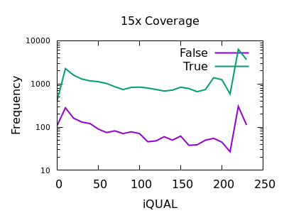
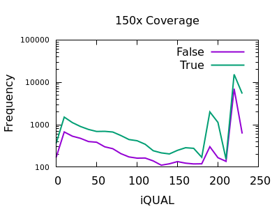
VCF Call Quality

We may produce a histogram from outdir/0003.vcf (true) and outdir/0001.vcf (false) to compare the distributions of the DP (depth) field. This may be either an INFO or a FORMAT field, but for simplicitly we are restricting this guide to a single sample and using INFO.

bcftools query -i 'TYPE="SNP"' -f '%QUAL\n' isec/0001.vcf > QUAL_1
bcftools query -i 'TYPE="SNP"' -f '%QUAL\n' isec/0003.vcf > QUAL_3

These files may be turned into histograms with a simple perl script or whatever language you prefer:

perl -MPOSIX -lane '$h{POSIX::round($F[0]/10)}++; END {@k=sort {$a <=> $b} (keys %h);for ($i=@k[0]; $i <= @k[-1]; $i++) {print $i*10,"\t",$h{$i}+0}}' QUAL_1 > QUAL_1_hist
perl -MPOSIX -lane '$h{POSIX::round($F[0]/10)}++; END {@k=sort {$a <=> $b} (keys %h);for ($i=@k[0]; $i <= @k[-1]; $i++) {print $i*10,"\t",$h{$i}+0}}' QUAL_3 > QUAL_3_hist

(Note if you are also going to be selectively filtering for high quality variants only, then you may wish to amend the “bcftools query” command above to -i 'TYPE="SNP" && QUAL >= 30' to see how the various metrics work in conjunction with quality filtering.)

Finally we can plot them in gnuplot, using a log scale as the disparity in sample sizes is very significant and attempting to normalise by total sample size may also mislead us.

$ gnuplot
gnuplot> set logscale y
gnuplot> plot \
    "QUAL_1_hist" with lines lw 2 title "False", \
    "QUAL_3_hist" with lines lw 2 title "True"

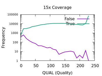
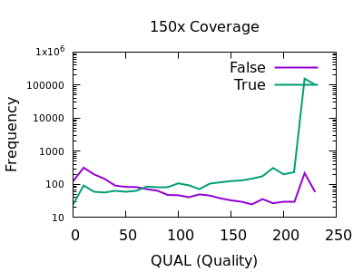
There are some strange spikes at very high values, but overall the trend is as we’d hope with an enrichment for false calls at low quality and for true calls at high quality.

At deep depths, we see a clear point of around 60 or below where calls are more likely to be incorrect than correct, but there are still a significant number of correct calls (log-odds of -0.5 equates to around 30:70 split in true:false).

For shallow depths, all quality values still are still more likely correct calls than incorrect.

Ultimately the threshold for filtering will depend on your application and whether high recall (low false negatives) is more important than high precision (low false positives).

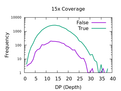
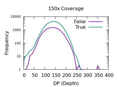
Depth

The sequencing depth may vary considerably across the sample. If we have a very sudden increase in depth, then it is possibly an indication of misalignment or an additional repeat copy in this sample vs the reference. Such cases can lead to incorrect calls, which are often extremely confident due to the high depth.

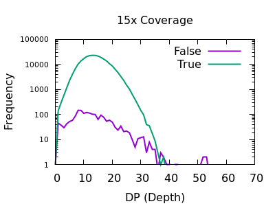
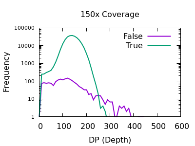
We see a sharp spike in depth for the true variants somewhere around the expected average depth. The false variants have a broader distribution with long tails.

The filter value obviously depends on the average depth, but filtering at some multiple of that can be powerful. For example 2 times the depth may be a reasonable starting point. We see here that perhaps DP > 35 will work well on the shallow data and DP > 250 for the deep data. These are not too far off doubling the depth (30 and 300).

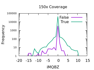
Mapping Quality

In a heterozygous call with one allele matching the reference, the distribution of mapping qualities for sequences matching REF versus those matching ALT may differ due to reference bias. This is to be expected, however a large difference in these distributions may be indicative of a false call. We have a Mann-Whitney U test available to compare these distributions. These are normalised into a Z-score, indicating the number of multiples of standard deviation above or below the mean. This is saved in the MQBZ INFO tag.

Normalised plots of these distributions can be seen here.

Note in bcftools 1.12 and earlier this is expressed as a probability value, so filter rules will need to check against very small values, such as MQB < 1e-5.

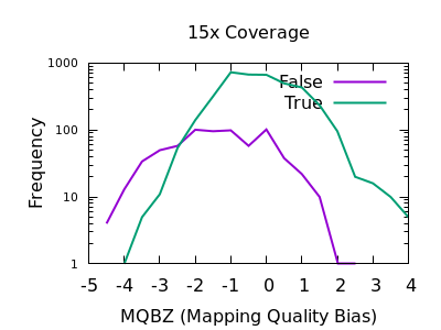
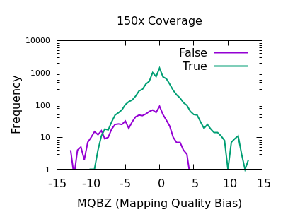
While there is a large overlap between the false and true distributions, at both low and high depth there is a clear shifting left for false variants. Unfortunately the correct filtering offset does also seem to be depth dependent. Filters of MQBZ < -4 would be appropriate for shallow data, and perhaps -9 for deep.

SNP Base Quality

Individual base qualities should have comparable distributions between REF and ALT. I bias here indicates the SNP may be a systematic error caused by a specific sequence motif.

Note in bcftools 1.12 and earlier this is expressed as a probability value, so filter rules will need to check against very small values, such as BQB < 1e-5.

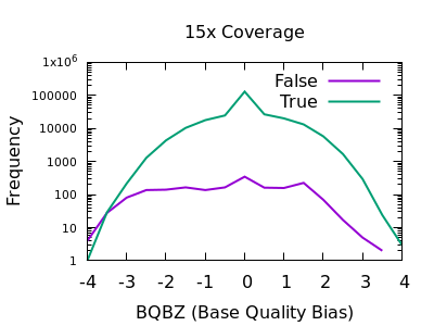
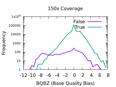
There is a slight skew towards lower BQBZ values for both low and high depth, with a more noticable discrimination at depth. The useful threshold varies slightly by depth.

%-(3.1 + DP/40)

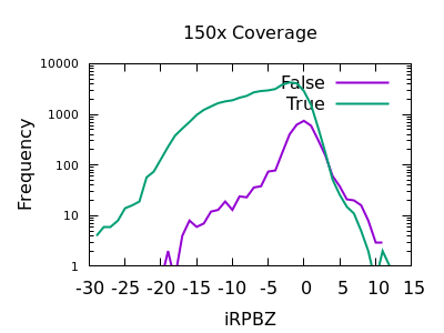
Position

The position of a variant within the reads can matter. We should expect reads to be aligned fairly randomly, and thus variants to be distributed randomly over the read. Reference bias alignment artifacts tend to be enriched for the ends of reads where a substitution near the read end is usually preferable to an indel to achieve optimal score (as alignments are pair-wise against the reference rather than against the other sequences within in the sample).

The RPBZ statistic is a Mann-Whitney U test represented as a Z-score (the distance from the mean expressed in units of the standard deviation) describing the difference in read position distributions of REF and ALT calls. As MQBZ this cannot be calculated for many SNPS, but where possible it can help spot false calls due to reference bias.

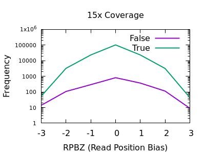
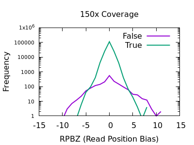
At shallow depth there isn’t any discrimination power between false and true variants. It’s more likely to be wrong at the extreme ends of the distribution, but it’s never more likely wrong than correct. At deep data however the statistic becomes far more powerful.

The plots are largely symmetric so a filter of e.g. RPBZ < -5 || RPBZ > +5 may work.

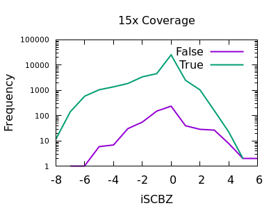
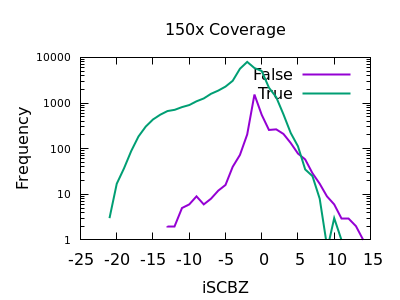
Soft-clips

A multitude of sequence alignments having soft-clipped bases may be indicative or a bad alignment, perhaps caused by reference bias again. The SCBZ is a Mann-Whitney U Z-score for the relative distribution of length of soft-clip within the proximity of the variant.

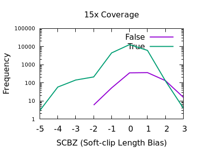
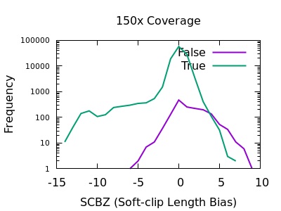
This test shows a sharp increase to the right end of the distribution for false variants. As with some other tests, the exact cutoff point is dependent on the depth of the sample.

A filter of SCBZ > 3 or SCBZ > 4 would be appropriate for this data.

Strand bias

This statistic is not enabled by default, but can be added with the -a FORMAT/SP option of bcftools mpileup.

The plots below are normalises, and truncated in X.

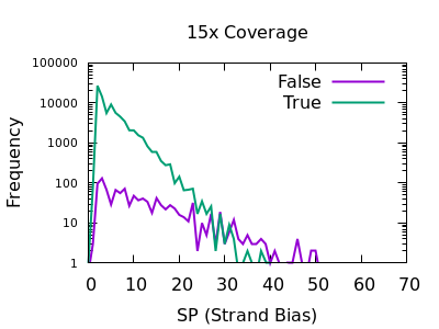
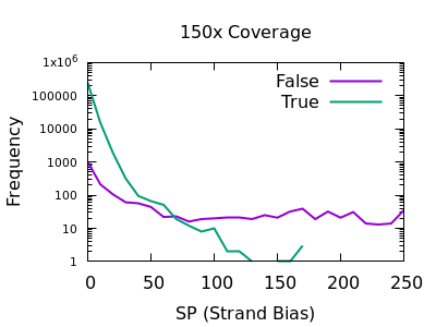
Both true and false variants have a sharp decay, but the tail is considerably longer for false variants. The test is still quite powerful for shallow data too.

As with some other metrics, the threshold is very depth specific, indicating FORMAT/SP > 100 for the 150x data and FORMAT/SP > 32 for the 15x data.

Putting it all together

While each test does not have a huge power to separate true from false variants, some of the indicators may not be strongly correlated so combining them together in a single clause can give a significant boost. If we are filtering out things that match our patterns, then we should combine with logical OR. For example the shallow data may use:

bcftools view -e 'QUAL <= 10 || DP > 35 || MQBZ < -3 || RPBZ < -3 || RPBZ > 3 || FORMAT/SP > 32 || SCBZ > 3' in.vcf

with the deep data using:

bcftools view -e 'QUAL <= 10 || DP > 250 || MQBZ < -3 || RPBZ < -3 || RPBZ > 3 || FORMAT/SP > 100 || SCBZ > 6' in.vcf

Note it’s possible to construct some filtering rules that adjust these thresholds according to the local depth of the data. This is challenging to optimise, but an example could be:

bcftools view -e "QUAL < $qual || DP>2*$DP || MQBZ < -(3.5+4*DP/QUAL) || RPBZ > (3+3*DP/QUAL) || RPBZ < -(3+3*DP/QUAL) || FORMAT/SP > (40+DP/2) || SCBZ > (2.5+DP/30)"

Where $qual is the desired quality threshold and $DP is the average sequencing depth.

It’s also worth noting that a lot of these tests filter the same variants, so we may wish to pick a good discriminator, such as MQBZ, and then filter on this prior to generating other plots such as RPBZ and SCBZ. Or we may wish to experiment with combinations such as summing. This article is not a complete tutorial, but aims to explain the ways you can experiment with filtering your own files.

Finally we can visualise the overall impact of our filtering by plotting at different QUAL thresholds from 0 to 200 in increments of 10 and displaying false positives vs false negatives, with and without the other filtering elements. Obviously this needs a good quality known truth set to be able to distinguish the variants. Doing this we see the combined power of the additional statistics. The below figure is for a 60x subsampling of GIAB HG002 chr1, showing SNP counts only.

The ideal position in this plot is the bottom left hand corner, with as few false positives (high precision) and few false negatives (high recall) as possible. We see the green filtered plot mainly moves leftwards, indicating a significant reduction in false positives with a very marginal change in false negatives.

InDel post-call filtering

Insertions and deletions use different INFO and FORMAT fields to SNPs and so need their own set of filter rules.

Applying similar strategies to above we can test the various INDEL statistics available.

Quality

Unfortunately the QUAL field really doesn’t seem particularly beneficial for indel filtering. There is perhaps a slight change in slope between true and false, meaning the cumulative numbers for variants above a specific QUAL may change, but it isn’t a particularly powerful metric.

Depth

As with SNPs, the total depth can be assessed via the INFO/DP field.

Unlike SNPs however the discrimination between true and false indels is weak. However the same depth filtering values of 35 and 250 (or 2x average depth if you just want a guess at a starting point) look to still apply.

Number of reads confirming an insertion or deletion

This field is specific to indels: the INFO/IDV metric.

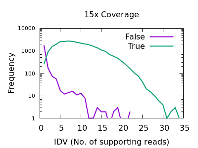
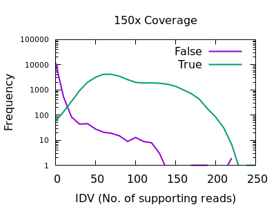
There is a very sharp drop in accuracy for low IDV values. A single read is quite unreliable, and a minimum of 2 would be recommended. Note earlier bcftools releases had a default of 1 (it is now 2), but this can also be adjusted with the mpileup -m 2 option.

Fraction of reads confirming an insertion or deletion

The INFO/IMF field is a fraction of the total reads matching an indel. This is a more useful metric than IDV for particularly deep data sets. It can also be controlled by the mpileup -F FLOAT option.

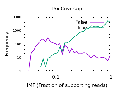
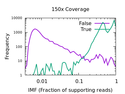
Note in this plot the X axis is also logarithmic, as the bulk of the discrimination power is in the very low fractions. For both data sets however IMF < 0.1 looks to be a suitable filter option.

Read Position Bias

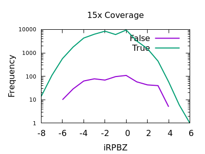
The RPBZ INFO field has an enrichment for false variants at above 6 or 7, although with shallow data this generally isn’t reached.

Soft-clip Bias

As for RPBZ, the SCBZ INFO field also has an enrichment for false variants at high values, above 8 or so for deep data.

There is some overlap with RPBZ too, but summing the two fields together before filtering works well. For example RPBZ + SCBZ > 9.

Mapping Quality Bias

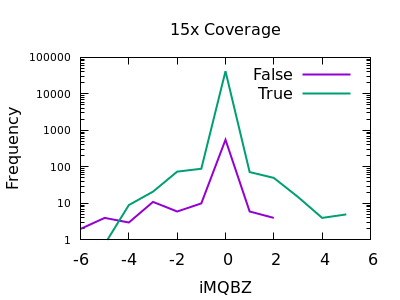
This isn’t as strong a selector as for SNPs, but the overall shape is consistent with extreme low values being more likely to be false calls. The cutoff point is very depth specific (as it is with SNPs).

Putting it all together

On a file containing indels, we can combine the various filter options together. Which parameters you use will depend on depth, but an attempt at a depth agnostic approach that works OK may be as follows:

bcftools view -e "IDV < 2 || \
    IMF < 0.02+(($qual+1)/($qual+31))*(($qual+1)/($qual+31))/4 || \
    DP > ($DP/2) * (1.7 + 12/($qual+20)) || \
MQBZ < -(5+DP/20) || RPBZ+SCBZ > 9" in.vcf

Note the QUAL column is completely absent in this filter rule as it simply isn’t robust enough (currently) for indel filtering.

Note if you’re going to be filtering heavily, favouring precision over recall, then you may wish to down-weight the initial likelihood of indels being called using e.g. --indel-bias 0.75. Conversely if you want as high a recall as possible, at the cost of some precision accuracy, boosting this with e.g. --indel-bias 2.0 may help. These are calling parameters that may have a better outcome than simply filtering. (No filter can ever generate more calls.)

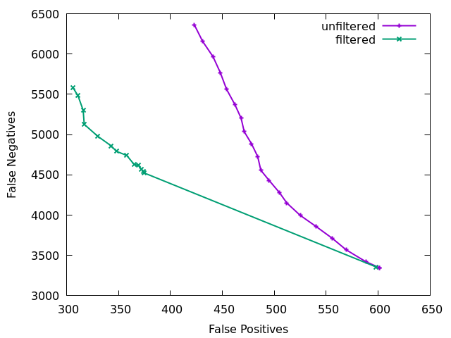
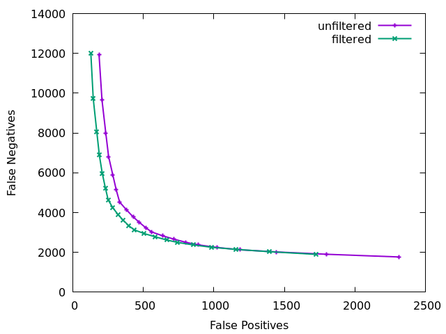
The above plot is showing false negatives (missing indels) vs false positives (incorrect indel calls) on a low 15x depth data set with and

without indel filtering. The effect is quite clear. The initial large jump from the first to second point comes primarily from needing at least 2 sequences (IDV<2) to at least 3 (IDV<3). The unfiltered plot is just using QUAL as a filter rule, which does give a slope trading FP and FN, but as discussed above is a rather poor filter. QUAL is unused in the filter plot.

Combined SNP and INDEL filtering

We now have one set of rules that work on SNPs and another that work on INDELs. We can either split our file up (e.g. `bcftools view -i ‘TYPE=”SNP”’) into SNP-only and INDEL-only, or we can combine the rules together.

This is possible, but it gets rather unwieldy.

The basic logic, assuming we are still using exclusion (filter-out) rules, would be:

bcftools view -e "(TYPE="SNP" && $snp_rule) || (TYPE="INDEL" && $indel_rule)" in.vcf

Copyright © 2023 Genome Research Limited (reg no. 2742969) is a charity registered in England with number 1021457. Terms and conditions.